

What is feature importance?
One of the key aspects in the process of creating a machine learning (ML) model is selecting appropriate, relevant features. In the process of assessing the input variable’s relevance, feature importance comes very handy. The goal of this process is to score each of the input variables.
The higher the score is, the more useful a specific feature was in the production of a result. One might ask why this process is important? There are multiple reasons. First and foremost, feature importance comes in extremely useful in selecting relevant features for our model.
It is crucial because it has a significant impact on the obtained solution. It is hard to expect a model that uses irrelevant features to be able to produce meaningful predictions. Apart from obtaining results, the issue of understanding data-driven solutions also plays a key role [1].
Clients often require an explanation of the prediction process. Not to mention the fields in which the interpretation of ML solutions is a strict requirement. A perfect example of such applications is those related to the medicine and banking sector.
In the case of medical implementation of artificial intelligence, domain experts must often confirm the correctness of the model’s output before it is used (think about cancer or any other severe illness diagnosis). It is especially the case if the prediction surprised them. [2]
The banking sector is another example of the branch in which the ability to interpret models is crucial. In some countries, there is a legal obligation to provide customers with an explanation regarding a decision related to credit approval. Finally, due to the abandonment of redundant features, ML solutions become much simpler while maintaining high performance.
Thus, according to Occam’s razor rule, the idea of “simplicity is a sign of truth” and so if the metric related to the specific solution is equal or highly similar between simple and complex models, then the latter is less preferable. Furthermore, having an interpretable model is also highly beneficial for convincing artificial intelligence skeptics and increasing the chances of implementation of data-driven solutions.
A potential problem
Let us imagine the following scenario, I am an eager data scientist with a regression problem task. As an eager data scientist I cannot wait for starting to build my machine learning model using all variables included in the dataset. I spent weeks performing feature engineering, trying out multiple models with various settings using hyperparameter tuning, and setting up a pipeline that combined all taken steps.
Unfortunately, the results are still not satisfactory, and I asked myself what did I do wrong? It turned out that my model consisted of some irrelevant features, which not only didn’t improve results but reduced the overall model performance. If I had taken the time to check feature importance, before jumping into the model right away, I would have not wasted valuable time.
How feature importance can be assessed with the help of python?
Now is probably the time in which the question of how one can check the importance of input features arises. It is mainly dependent on the type of model we are using, however, some techniques might be applied regardless of the used model (for example permutation feature importance).
- Linear models
In terms of linear models, this process is straightforward. While fitting our model, the coefficients to the specific features are calculated. These coefficients tell us how much our target variable increases (or decrease in the case of coefficient negative value) when our feature will increase by one. However, there is also an issue that needs to be considered.
The obtained coefficients indicate the feature importance of corresponding features under the assumption that features are on the same scale, which is not the case here (Values from the “tax” column differ from 187 to 711, whereas values of the “nox” column are in the range from 0.35 to 0.87). That is why, to cope with this issue, data should be standardized before fitting them into our linear regression model [3].
To get the coefficients of the linear model, we just need to extract attribute coef_ from our trained model. Based on these extracted values, one can plot the following bar plot: (An important note here, to show the significance of the variables better I plotted their absolute values, not the real ones).
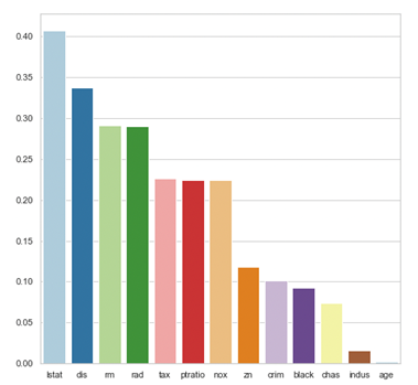
Figure 1 The barplot with corresponding feature importance values
As it can be seen, features in our model vary significantly in their importance. The two most important ones are “lstat” which indicates the lower status of the population and the “dis” which tells us about the weighted mean of distances to five Boston employment centers.
On the other hand, the least important variables are “age” and “Indus” which inform us about the proportion of owner-occupied units as well as non-retail business acres per town respectively. These coefficients also intuitively make sense. One can suspect that the information about location and the neighbourhood’s financial status provides more insights into the model than the proportion of non-retail businesses.
- Tree-based models
In terms of tree-based models, there are multiple ways to examine the feature importance of the used variables. In this section, I would like to focus on the Gini Importance and Permutation Importance.
Gini importance is a measure that is defined by an average of the total decrease in node impurity which is weighted by the probability of reaching this node. This probability is calculated simply by the proportion of samples that reach this node to build a decision tree.
There is an issue here that the impurity-based feature importance has a biased towards the features that contain a lot of unique values [4]. Because of that, this kind of feature might be overvalued in comparison to the categorical features which might be more informative. That is why to cope with this limitation we can use permutation importance.
One of the most important properties of feature importance is the fact that it can be used to access the feature importance of any estimator if the used data has a tabular form [6]. This metric measures the difference between the error obtained with an initial distribution of a variable and the error when this variable has been shuffled (all other variables are fixed).
The idea is that if the described difference is significant then we assume that this feature is important concerning our model. The examination of feature importance with the hand of permutation importance is incredibly straightforward.
We can import the function from the scikit learn “inspection” module directly and use it on our model with data (it can be performed both with training as well as validation dataset, but performing feature importance on training dataset might lead to overfitting).
- Neural Networks
Interpretation of Neural Networks is a challenging task due to the high parameters number and often complex processes related to feature engineering. There is a lot of research that focuses on looking at what neural networks are learning.
To answer this question, researchers want to link the deep learning outputs with its inputs. Several methods try to achieve this goal, such as Sensitivity Analysis or Taylor decomposition. However, both techniques have shortcomings caused by the focus on the local variations and an extensively high amount of negative relevance respectively.
That is why the more widely used methods are backward propagation techniques [5]. Layerwise Relevance Propagation (LRP) belongs to this method’s family. To explain the idea behind this technique I’d like to draw attention to the following picture:
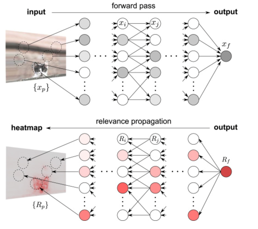
Figure 2 Graphical representation of LRP technique [5]
The first phase of the process is the same for any neural network, having an input (in this case a photo) net performs a forward pass and consequently produces an output. In the case of classification problems, the output often indicates the probability of a label being in the specified class.
This value is then interpreted by LRP as a relevance value. Having this value, we are propagating backward by calculating the relevance value of each node concerning its corresponding value from the next layer. This process takes place until we get to the original input, in which we can create a heatmap of input relevance concerning calculated relevance values.
Conclusions & summary
To sum up, the interpretation of machine learning models plays a key role. Not only does it provide us with an opportunity to increase the model performance, but it is also often a crucial part of the solution. The technique that provides information regarding feature importance depends heavily on the used algorithm.
References:
- Zien, A., Krämer, N., Sonnenburg, S., Rätsch, G. (2009). The Feature Importance Ranking Measure, Springer 5782 (2009).
- Adrien Bibal, Benoît Frénay, “Interpretability of Machine Learning Models and Representations: An Introduction”, European Symposium on Artificial Neural Networks, Computational Intelligence and Machine Learning (2016).
- Chirag Goyal, “Standardized vs unstandardized regression coefficient”, Analytics Vidhya, March 2021, Link: https://www.analyticsvidhya.com/blog/2021/03/standardized-vs-unstandardized-regression-coefficient/
- Scikit- learn document, Link: https://scikit-learn.org/stable/modules/permutation_importance.html#permutation-importance
- Grégoire Montavon, Wojciech Samek, Klaus-Robert Müller, “Methods for interpreting and understanding deep neural networks”, Digital Signal Processing 73 (2018).
- Grégoire Montavon, Sebastian Lapuschkin, Alexander Binder, Wojciech Samek, Klaus-Robert Müller, “Explaining nonlinear classification decisions with deep Taylor decomposition”, Pattern Recognition 65 (2017).